A fixed effect model is a statistical model that includes fixed effects, which are parameters that are estimated to be constant across different groups.
Example [Panel Data]: In the context of panel data, fixed effects are parameters that are constant across different individuals or time. The typical model example is given by the following equation:
where \(Y_{it}\) is the dependent variable for individual \(i\) at time \(t\), \(X_{it}\) is the independent variable, \(\beta\) is the coefficient of the independent variable, \(\alpha_i\) is the individual fixed effect, \(\psi_t\) is the time fixed effect, and \(\varepsilon_{it}\) is the error term. The individual fixed effect \(\alpha_i\) is a parameter that is constant across time for each individual, while the time fixed effect \(\psi_t\) is a parameter that is constant across individuals for each time period.
Note however that, despite the fact that fixed effects are commonly used in panel setting, one does not need a panel data set to work with fixed effects. For example, cluster randomized trials with cluster fixed effects, or wage regressions with worker and firm fixed effects.
In this “quick start” guide, we will show you how to estimate a fixed effect model using the PyFixest package. We do not go into the details of the theory behind fixed effect models, but we focus on how to estimate them using PyFixest.
Read Sample Data
In a first step, we load the module and some synthetic example data:
import matplotlib.pyplot as pltimport numpy as npimport pandas as pdtry:from lets_plot import LetsPlot _HAS_LETS_PLOT =TrueexceptImportError: _HAS_LETS_PLOT =Falsefrom marginaleffects import slopes, avg_slopesimport pyfixest as pfif _HAS_LETS_PLOT: LetsPlot.setup_html()plt.style.use("seaborn-v0_8")%load_ext watermark%config InlineBackend.figure_format ="retina"%watermark --iversionsdata = pf.get_data()data.head()
We see that some of our columns have missing data.
OLS Estimation
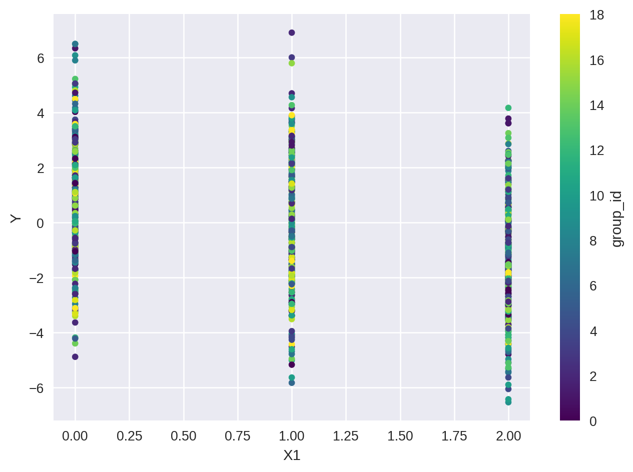
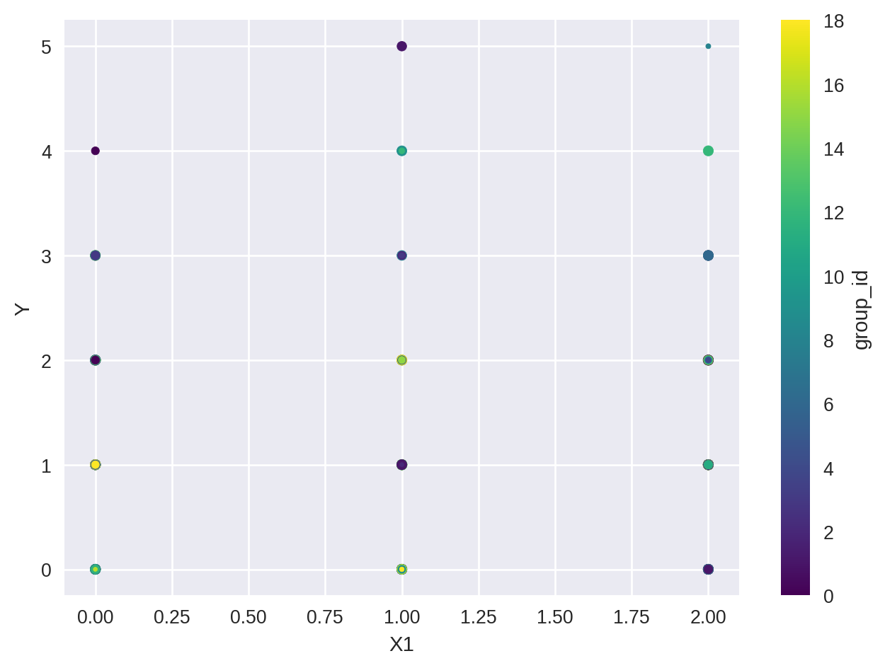
We are interested in the relation between the dependent variable Y and the independent variables X1 using a fixed effect model for group_id. Let’s see how the data looks like:
We can estimate a fixed effects regression via the feols() function. feols() has three arguments: a two-sided model formula, the data, and optionally, the type of inference.
fit = pf.feols(fml="Y ~ X1 | group_id", data=data, vcov="HC1")type(fit)
OMP: Info #276: omp_set_nested routine deprecated, please use omp_set_max_active_levels instead.
pyfixest.estimation.models.feols_.Feols
The first part of the formula contains the dependent variable and “regular” covariates, while the second part contains fixed effects.
feols() returns an instance of the Fixest class.
Inspecting Model Results
To inspect the results, we can use a summary function or method:
Significance levels: * p < 0.05, ** p < 0.01, *** p < 0.001. Format of coefficient cell: Coefficient (Std. Error)
Alternatively, the .summarize module contains a summary function, which can be applied on instances of regression model objects or lists of regression model objects. For details on how to customize etable(), please take a look at the dedicated vignette.
You can access individual elements of the summary via dedicated methods: .tidy() returns a “tidy” pd.DataFrame, .coef() returns estimated parameters, and se() estimated standard errors. Other methods include pvalue(), confint() and tstat().
Coefficient
X1   -12.233634
Name: t value, dtype: float64
fit.confint()
2.5%
97.5%
X1
-1.182467
-0.85555
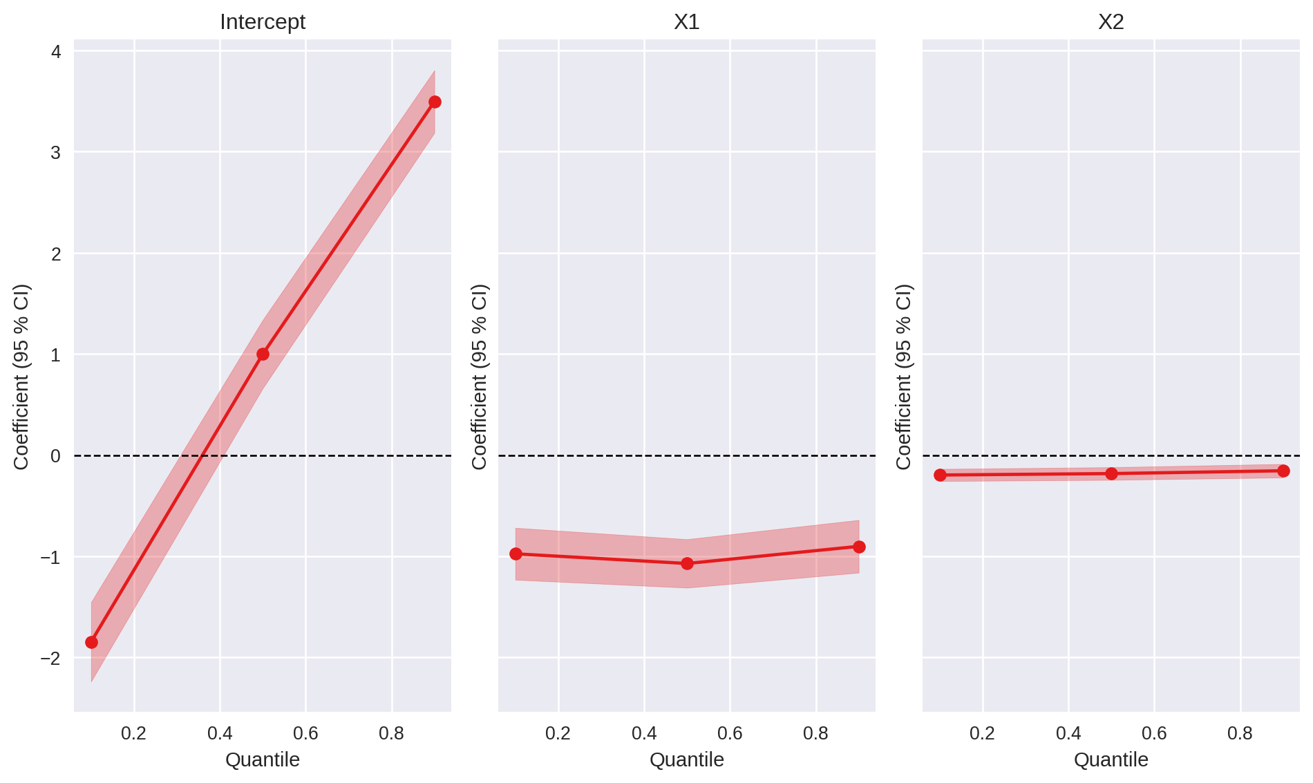
Last, model results can be visualized via dedicated methods for plotting:
fit.coefplot()# or pf.coefplot([fit])
How to interpret the results?
Let’s have a quick d-tour on the intuition behind fixed effects models using the example above. To do so, let us begin by comparing it with a simple OLS model.
We can compare both models side by side in a regression table:
pf.etable([fit, fit_simple])
Y
(1)
(2)
coef
X1
-1.019*** (0.083)
-1.000*** (0.082)
Intercept
0.919*** (0.112)
fe
group_id
x
-
stats
Observations
998
998
R2
0.137
0.123
Significance levels: * p < 0.05, ** p < 0.01, *** p < 0.001. Format of coefficient cell: Coefficient (Std. Error)
We see that the X1 coefficient is -1.019, which is less than the value from the OLS model in column (2). Where is the difference coming from? Well, in the fixed effect model we are interested in controlling for the feature group_id. One possibility to do this is by adding a simple dummy variable for each level of group_id.
This is does not scale well! Imagine you have 1000 different levels of group_id. You would need to add 1000 dummy variables to your model. This is where fixed effect models come in handy. They allow you to control for these fixed effects without adding all these dummy variables. The way to do it is by a demeaning procedure. The idea is to subtract the average value of each level of group_id from the respective observations. This way, we control for the fixed effects without adding all these dummy variables. Let’s try to do this manually:
We get the same results as the fixed effect model Y1 ~ X | group_id above. The PyFixest package uses a more efficient algorithm to estimate the fixed effect model, but the intuition is the same.
Updating Regression Coefficients
You can update the coefficients of a model object via the update() method, which may be useful in an online learning setting where data arrives sequentially.
To see this in action, let us first fit a model on a subset of the data:
Supported covariance types are “iid”, “HC1-3”, CRV1 and CRV3 (up to two-way clustering).
Why do we have so many different types of standard errors?
The standard errors of the coefficients are crucial for inference. They tell us how certain we can be about the estimated coefficients. In the presence of heteroskedasticity (a situation which typically arises with cross-sectional data), the standard OLS standard errors are biased. The pyfixest package provides several types of standard errors that are robust to heteroskedasticity.
iid: assumes that the error variance is spherical, i.e. errors are homoskedastic and not correlated (independent and identically distributed errors have a spherical error variance).
CRV1 and CRV3: cluster robust standard errors according to Cameron, Gelbach, and Miller (2011). See A Practitioner’s Guide to Cluster-Robust Inference. For CRV1 and CRV3 one should pass a dictionaty of the form {"CRV1": "clustervar"}.
Inference can be adjusted “on-the-fly” via the .vcov() method:
Panel Data Example: Causal Inference for the Brave and True
In this example we replicate the results of the great (freely available reference!) Causal Inference for the Brave and True - Chapter 14. Please refer to the original text for a detailed explanation of the data.
The objective is to estimate the effect of the variable married on the variable lwage using a fixed effect model on the entity variable nr and the time variable year.
panel_fit = pf.feols( fml="lwage ~ expersq + union + married + hours | nr + year", data=data_df, vcov={"CRV1": "nr + year"},)pf.etable(panel_fit)
lwage
(1)
coef
expersq
-0.006*** (0.000765)
union
0.073* (0.023)
married
0.048* (0.018)
hours
-0.000136** (0.000035)
fe
year
x
nr
x
stats
Observations
4,360
R2
0.631
Significance levels: * p < 0.05, ** p < 0.01, *** p < 0.001. Format of coefficient cell: Coefficient (Std. Error)
We obtain the same results as in the book!
Instrumental Variables (IV) Estimation
It is also possible to estimate instrumental variable models with one endogenous variable and (potentially multiple) instruments.
In general, the syntax for IV is depvar ~ exog.vars | fixef effects | endog.vars ~ instruments.
/Users/afischer/Documents/pyfixest/pyfixest/estimation/quantreg/quantreg_.py:77: FutureWarning:
           The Quantile Regression implementation is experimental and may change in future releases.
           But mostly, we expect the API to remain unchanged.
You can test multiple hypotheses simultaneously via the wald_test method.
fit = pf.feols("Y ~ X1 + X2 | f1", data=data)
For example, to test the joint null hypothesis of \(X_{1} = 0\) and \(X_{2} = 0\) vs the alternative that \(X_{1} \neq 0\) or \(X_{2} \neq 0\), we would run
Alternatively, suppose we wanted to test a more complicated joint null hypothesis: \(X_{1} + 2X_{2} = 2.0\) and \(X_{2} = 1.0\). To do so, we would define \(R\) and \(q\) as
/Users/afischer/Documents/pyfixest/pyfixest/estimation/models/feols_.py:1222: UserWarning: Distribution changed to chi2, as R is not an identity matrix and q is not a zero vector.
Generalized Linear Models (GLMs) with Fixed Effects
PyFixest supports GLMs (logit, probit, gaussian) with high-dimensional fixed effects via pf.feglm(). Fixed effects are specified after the | symbol, just like in feols().
/Users/afischer/Documents/pyfixest/.pixi/envs/docs/lib/python3.12/site-packages/marginaleffects/comparisons.py:71: UserWarning: For this pyfixest model, marginaleffects cannot take into account the uncertainty in fixed-effects parameters. Standard errors are disabled and vcov=False is enforced.
shape: (1, 3)
term
contrast
estimate
str
str
f64
"X1"
"dY/dX"
-1.016344
Please take a look at the marginaleffects book to learn about other transformations that the marginaleffects package supports.
Multiple Estimation
PyFixest supports a range of multiple estimation functionality: sw, sw0, csw, csw0, and multiple dependent variables. The meaning of these options is explained in the Multiple Estimations vignette of the fixest package:
sw: this function is replaced sequentially by each of its arguments. For example, y ~ x1 + sw(x2, x3) leads to two estimations: y ~ x1 + x2 and y ~ x1 + x3.
sw0: identical to sw but first adds the empty element. E.g. y ~ x1 + sw0(x2, x3) leads to three estimations: y ~ x1, y ~ x1 + x2 and y ~ x1 + x3.
csw: it stands for cumulative stepwise. It adds to the formula each of its arguments sequentially. E.g. y ~ x1 + csw(x2, x3) will become y ~ x1 + x2 and y ~ x1 + x2 + x3.
csw0: identical to csw but first adds the empty element. E.g. y ~ x1 + csw0(x2, x3) leads to three estimations: y ~ x1, y ~ x1 + x2 and y ~ x1 + x2 + x3.
Additionally, we support split and fsplit function arguments. > - split allows to split a sample by a given variable. If specified, pf.feols() and pf.fepois() will loop through all resulting sample splits. > - fsplit works just as split, but fits the model on the full sample as well.
If multiple regression syntax is used, feols() and fepois returns an instance of a FixestMulti object, which essentially consists of a dicionary of Fepois or Feols instances.
<pyfixest.estimation.FixestMulti_.FixestMulti at 0x33c9533b0>
multi_fit.etable()
Y
(1)
(2)
(3)
coef
X1
-1.000*** (0.082)
-0.949*** (0.067)
-0.919*** (0.06)
Intercept
0.919*** (0.112)
fe
f2
-
-
x
f1
-
x
-
f1
-
-
x
stats
Observations
998
997
997
R2
0.123
0.437
0.609
Significance levels: * p < 0.05, ** p < 0.01, *** p < 0.001. Format of coefficient cell: Coefficient (Std. Error)
You can access an individual model by its name - i.e. a formula - via the all_fitted_models attribute.
multi_fit.all_fitted_models["Y ~ X1"].tidy()
Estimate
Std. Error
t value
Pr(>|t|)
2.5%
97.5%
Coefficient
Intercept
0.918518
0.111707
8.222580
6.661338e-16
0.699310
1.137725
X1
-1.000086
0.082420
-12.134086
0.000000e+00
-1.161822
-0.838350
or equivalently via the fetch_model method:
multi_fit.fetch_model(0).tidy()
Model: Y ~ X1
Estimate
Std. Error
t value
Pr(>|t|)
2.5%
97.5%
Coefficient
Intercept
0.918518
0.111707
8.222580
6.661338e-16
0.699310
1.137725
X1
-1.000086
0.082420
-12.134086
0.000000e+00
-1.161822
-0.838350
Here, 0 simply fetches the first model stored in the all_fitted_models dictionary, 1 the second etc.
Objects of type Fixest come with a range of additional methods: tidy(), coef(), vcov() etc, which essentially loop over the equivalent methods of all fitted models. E.g. Fixest.vcov() updates inference for all models stored in Fixest.
/var/folders/98/c353q4p95v5_fz62gr5c9td80000gn/T/ipykernel_42193/2324653916.py:20: DeprecationWarning: The function `_relabel_expvar` is deprecated as we have adjusted the naming of variables interacted via the i() operator with pyfixest 0.50. For regression tables, please rely on the `labels` and `cat_template` arguments of `pf.etable()` instead.
The event_study() function provides a common API for several event study estimators.